Transformer: From Principle to Implementation

Overview

Transformer 的提出主要解决 RNN 的三个问题：

1. 最小化每层的计算复杂度。
2. 最小化任何一对词间的路径长度：RNN 从左到右顺序编码，需要 $\mathcal{O}(N)$ 步才能让远距离的词间进行交互。这意味着 RNN 难以学习长距离依赖，由于梯度问题。
3. 最大化可并行化的计算量：RNN 前向与反向传播均有 $\mathcal{O}(N)$ 步不可并行的计算，无法充分利用 GPU, TPU 等

假设 $N$ 为序列长度，$D$ 为表示维度。recurrent 和 self-attention 的每层复杂度如下表所示：

Layer Type	Complexity per Layer
Self-Attention	$\mathcal{O}(N^{2} \cdot D)$
Recurrent	$\mathcal{O}(N \cdot D^{2})$

当 $N \ll D$ 时，Transformer 的每层复杂度比 RNN 低。

以机器翻译任务为例，Transformer 的输入与输出如下：

• Input: sentences in the source language. E.g. I am a student (in English)
• Output: sentences in the target language. E.g. 我是一个学生 (in Chinese)

Transformer 的整体架构如下图所示：

Transformer 主要由两个组件 (i.e. encoder & decoder) 构成，每个组件都由多个相同的层堆叠而成 (原论文中，encoder 与 decoder 层数均为 $6$)。直观地，两个组件的作用如下：

• Encoder: 给定输入序列，转换成中间表示，捕获序列中的依赖关系
  • Input: 输入序列
  • Output: 输入序列的中间表示
• Decoder: 给定 encoder 输出的源序列中间表示，生成目标序列
  • Input: Encoder 的输出
  • Output: 目标序列的概率分布

Encoders

每层 encoder 结构上完全一致 (但权重并不共享)，均由两个子层构成：

1. 多头自注意力机制 (multi-head self-attention)
2. 位置全连接前馈网络 (position-wise fully connected feed-forward network)

进入第一个 encoder 前，需要经过：

1. 嵌入层 (embedding layer)
2. 位置编码 (positional encoding)

对两个子层，使用两个 trick (对应于架构图中的 Add & Norm):

1. 残差连接 (residual connection)
2. 层归一化 (layer normalization)

为了使用 residual connection，模型 (包括 encoder 与 decoder) 所有的子层以及 embedding 层的输出维度均相同 (原论文中设置为 $D_{\text{model}} = 512$)。

接下来，后文仍然以机器翻译任务为例，自底向上介绍 encoder 的各个组件，最后介绍 Add & Norm 等 trick。

Embedding Layer

• Input: a sentence in the source language $X = x_{1}x_{2} \ldots x_{N}$, where $x_{i}$ is the $i$-th word in the sentence with $N$ words.
• Output: an embedding matrix $\mathbf{X} = [\mathbf{x}_{1}, \mathbf{x}_{2}, \ldots, \mathbf{x}_{N}] \in \mathbb{R}^{N \times D_{\text{model}}}$, where $\mathbf{x}_{i} \in \mathbb{R}^{D_{\text{model}}}$ is the $i$-th word embedding.

Positional Encoding

• Motivation: Transformer 没有使用 CNN, RNN，可以捕获单词语义信息，但无法捕获单词间的顺序与距离等位置信息
• Solution: 将位置编码向量添加到 encoder 与 decoder 底层的词嵌入向量中，二者维度相同

在原论文中，位置编码 $\mathbf{P} \in \mathbb{R}^{N \times D_{\text{model}}}$ 是通过正弦和余弦函数生成的：

$$\begin{aligned} \mathbf{P}_{pos, 2i} &= \sin\bigg(\frac{pos}{10000^{2i/D_{\text{model}}}}\bigg)\\ \mathbf{P}_{pos, 2i+1} &= \cos\bigg(\frac{pos}{10000^{2i/D_{\text{model}}}}\bigg) \end{aligned}$$

其中：

• $pos$: 单词位置索引
• $i$: 位置编码维度索引
• $D_{\text{model}}$: 词嵌入维度

接着，将位置编码向量与起始嵌入向量相加，得到新的输入嵌入：

$$\mathbf{X}^{\prime} = \mathbf{X} + \mathbf{P}$$

其中：$\mathbf{x}_{pos}^{\prime} = \mathbf{x}_{pos} + \mathbf{p}_{pos}$。为了便于表示，后文仍将 $\mathbf{X}^{\prime}$ 记为 $\mathbf{X}$

实现如下：

def precompute_pe(n_embd: int, n_positions: int) -> torch.Tensor:
    """Precompute positional encoding.

    Args:
        n_embd (int): Embedding dimension.
        n_positions (int): Maximum sequence length.

    Returns:
        torch.Tensor: Positional encoding of shape (n_positions, n_embd).
    """
    pe = torch.zeros(n_positions, n_embd)  # (n_positions, n_embd)
    pos = torch.arange(n_positions, dtype=torch.float32)  # (n_positions,)
    div_term = torch.exp(
        torch.arange(0, n_embd, 2, dtype=torch.float32)  # (n_embd // 2,)
        * -(torch.log(torch.tensor(10000.0)) / n_embd)
    )  # (n_embd // 2,)
    pos_div_term = pos.unsqueeze(-1) * div_term  # (n_positions, n_embd // 2)
    pe[:, 0::2] = torch.sin(pos_div_term)
    pe[:, 1::2] = torch.cos(pos_div_term)
    return pe


def apply_pe(x: torch.Tensor, pe_cache: torch.Tensor) -> torch.Tensor:
    """Apply positional encoding to input tensor.

    Args:
        x (torch.Tensor): Input tensor of shape (batch_size, seq_len, n_embd).
        pe_cache (torch.Tensor): Positional encoding of shape (n_positions, n_embd).

    Returns:
        torch.Tensor: Output tensor of shape (batch_size, seq_len, n_embd).
    """
    seq_len = x.size(1)  # actual sequence length
    n_positions = pe_cache.size(0)  # maximum sequence length
    # Truncate `pe_cache` to match the length of `x`
    if n_positions > seq_len:
        pe_cache = pe_cache[:seq_len, :]  # (seq_len, n_embd)
    return x + pe_cache.unsqueeze(0)  # (batch_size, seq_len, n_embd)

在训练或推理阶段，位置编码是固定的，与输入数据无关。因此，采用预计算的策略，即：对位置编码 $\mathbf{P}$ 提前计算，在相关模块 (nn.Module) 的构造方法 __init__ 中，通过 self.register_buffer() 缓存，避免重复计算。

Attention

Overview of Attention Mechanism

• Intuition: 序列中的某些部分往往更重要，注意力机制允许模型动态地关注主要信息，忽略次要信息。
• Solution: 通过计算 $\mathbf{Q}, \mathbf{K}, \mathbf{V}$ 实现

给出一个直观的比喻：假设你是一个图书管理员，你想寻找图书馆中某本符合你需求的书。

• Query (Q): 代表你的需求，描述了你在寻找什么样的书（比如 " 历史类书籍 "）。
• Key (K): 代表每本书的标签或描述，用于标明它们的内容（比如 " 历史 “、” 科学 “、” 文学 " 等）。
• Value (V): 代表书本的具体内容，也就是你真正需要获取的信息。

注意力机制的作用是：计算你的需求 (Query) 和每本书的标签 (Key) 之间的相似性，找到最符合需求的书籍，并根据相似度调整你对每本书内容 (Value) 的关注程度。

以 Seq2Seq 机器翻译任务为例，注意力机制的作用在于为目标语言中的每个单词选择性关注源语言的某些单词，与 Transformer 的 decoder 中的 Encoder-Decoder Attention 类似，而 encoder 中的 self-attention 与之略有差异。这两种注意力机制的 $\mathbf{Q}, \mathbf{K}, \mathbf{V}$ 来源归纳如下：

Mechanism	$\mathbf{Q}$	$\mathbf{K, V}$
Encoder-Decoder Attention	target language	source language
Self-Attention	source language	source language

Self-Attention

计算步骤如下：

第一步，对于每个单词 $\mathbf{x}_{i}$, 计算其 query, key, value

$$\begin{aligned} \mathbf{q}_{i} = (\mathbf{W}^{Q})^{\top}\mathbf{x}_{i} \\ \mathbf{k}_{i} = (\mathbf{W}^{K})^{\top}\mathbf{x}_{i} \\ \mathbf{v}_{i} = (\mathbf{W}^{V})^{\top}\mathbf{x}_{i} \end{aligned}$$

其中：

• $\mathbf{x}_{i} \in \mathbb{R}^{D_\text{model}}$
• $\mathbf{q}_{i}, \mathbf{k}_{i} \in \mathbb{R}^{D_{k}}$, $\mathbf{v}_{i} \in \mathbb{R}^{D_{v}}$
• $\mathbf{W}^{Q}, \mathbf{W}^{K} \in \mathbb{R}^{D_{\text{model}} \times D_{k}}$, $\mathbf{W}^{V} \in \mathbb{R}^{D_{v}}$

第二步，计算 query 和 key 间的注意力分数

$$e_{ij} = \mathbf{q}_{i} \mathbf{k}_{j}^{\top} \in \mathbb{R}$$

第三步，对注意力分数进行 softmax 归一化

$$\alpha_{ij} = \mathrm{softmax}(e_{ij}) = \frac{\exp(e_{ij})}{\sum_{k} \exp(e_{ik})}$$

第四步，对 value 使用注意力分数加权求和

$$\mathbf{z}_{i} = \sum_{j} \alpha_{ij} \mathbf{v}_{j}$$

Scaled Dot-Product Attention

• Motivation:
  • 相比加性注意力，由于矩阵乘法实现的优化，点积注意力计算时空复杂性更低
  • softmax 函数对输入的尺度非常敏感：
    • 输入值过大，输出趋于 $1$ 或 $0$，导致梯度消失
    • 输入值过小，输出趋于均匀分布，导致注意力机制无法有效捕捉相关性
• Solution: 引入合适的缩放因子 (scaling factor)，确保 softmax 的输入位于合理的范围

具体地，在计算注意力分数时，引入缩放因子 $D_{k}$：

$$e_{ij} = \frac{\mathbf{q}_{i} \mathbf{k}_{j}^{\top}}{\sqrt{D_{k}}} \in \mathbb{R}$$

为什么采用 $\frac{1}{\sqrt{D_{k}}}$ 进行缩放？假设 $\mathbf{q}, \mathbf{k} \sim \mathcal{N}(0,1)$, 则 $\mathrm{Var}(\mathbf{q} \cdot \mathbf{k}^{\top}) = \sqrt{D_{k}}$。为了使注意力分数方差保持在合理的范围内，将其缩放到方差为 $1$，即：$\mathrm{Var}(\frac{\mathbf{q} \cdot\mathbf{k}^{\top}}{\sqrt{D_{k}}}) = 1$

Vectorization for Self-Attention

现使用矩阵形式，重新描述自注意力机制：

$$\mathbf{Z} = \mathrm{Attention}(\mathbf{Q}, \mathbf{K}, \mathbf{V}) = \mathrm{softmax} \bigg( \frac{\mathbf{Q}\mathbf{K}^{\top}}{\sqrt{D_{k}}} \bigg)\mathbf{V}$$

其中：

• $\mathbf{Q} = \mathbf{X}\mathbf{W}^{Q} \in \mathbb{R}^{N \times D_{k}}$
• $\mathbf{K} = \mathbf{X}\mathbf{W}^{K} \in \mathbb{R}^{N \times D_{k}}$
• $\mathbf{V} = \mathbf{X}\mathbf{W}^{V} \in \mathbb{R}^{N \times D_{v}}$
• $\mathbf{X}, \mathbf{Z} \in \mathbb{R}^{N \times D_{\text{model}}}$

原论文中，$D_{k} = D_{v}$

Multi-Head Self-Attention

• Motivation: 关注不同位置的不同特征子空间，从而捕获序列中不同层次的依赖关系
• Solution: 对同一个输入序列进行多组并行注意力计算，对结果进行拼接和线性变换

计算公式如下：

$$\begin{aligned} \mathbf{Z} = \mathrm{MultiHead}(\mathbf{Q}, \mathbf{K}, \mathbf{V}) &= \mathrm{Concat}(\mathrm{head}_{1}, \ldots, \mathrm{head}_{H}) \mathbf{W}^{O} \\ \text{where} \ \mathrm{head}_{i} &= \mathrm{Attention}(\mathbf{Q}_{i}, \mathbf{K}_{i}, \mathbf{V}_{i}) \end{aligned}$$

其中：

• $\mathbf{Q}_{i} = \mathbf{X}\mathbf{W}^{Q_{i}} \in \mathbb{R}^{N \times D_{k}}$
• $\mathbf{K}_{i} = \mathbf{X}\mathbf{W}^{K_{i}} \in \mathbb{R}^{N \times D_{k}}$
• $\mathbf{V}_{i} = \mathbf{X}\mathbf{W}^{V_{i}} \in \mathbb{R}^{N \times D_{v}}$
• $\mathbf{W}^{O} \in \mathbb{R}^{HD_{v} \times D_{\text{model}}}$

原论文中，$H=8$, $D_{k} = D_{v} = D_{\text{model}} / H = 64$

由于多头注意力是并行计算，因此，计算开销与单头注意力相近。

实现如下：

class SelfAttention(nn.Module):

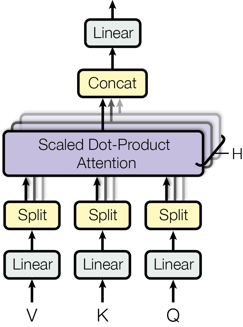
    def __init__(
        self,
        n_embd: int,
        n_head: int,
        attn_pdrop: float = 0.1,
        resid_pdrop: float = 0.1,
        bias: bool = True,
    ) -> None:
        """Initialize the module.

        Args:
            n_embd (int): Embedding dimension.
            n_head (int): Number of attention heads.
            attn_pdrop (float):
                Dropout probability for attention weights.
                Defaults to 0.1.
            resid_pdrop (float):
                Dropout probability for residual connections.
                Defaults to 0.1.
            bias (bool, optional):
                Whether to include bias terms when calculating k, q, v projections.
                Defaults to True.
        """
        super().__init__()
        assert n_embd % n_head == 0  # n_embd must be divisible by n_head
        # key, query, value projections for all heads, but in a batch
        self.c_attn = nn.Linear(n_embd, 3 * n_embd, bias=bias)
        # output projection
        self.c_proj = nn.Linear(n_embd, n_embd, bias=bias)
        # regularization
        self.attn_dropout = nn.Dropout(attn_pdrop)
        self.resid_dropout = nn.Dropout(resid_pdrop)
        self.n_head = n_head

    def forward(self, x: torch.Tensor) -> torch.Tensor:
        """Forward pass.

        Args:
            x (torch.Tensor): Input tensor of shape (B, T, C) where
                B is the batch size,
                T is the sequence length,
                C is the embedding dimension.

        Returns:
            torch.Tensor: Output tensor of shape (B, T, C).
        """
        # B: batch size, T: sequence length, C: embedding dimension (=n_embd)
        B, T, C = x.size()

        # calculate q, k, v for all heads in batch
        # (B, T, C) -> (B, T, 3C) -> (B, T, C) x 3
        q, k, v = self.c_attn(x).split(C, dim=-1)
        # move head dim forward to be the batch dim
        # (B, T, C) -> (B, T, nh, hs) -> (B, nh, T, hs)
        # C = nh * hs, where nh: number of heads, hs: head size,
        q = q.view(B, T, self.n_head, C // self.n_head).transpose(1, 2)
        k = k.view(B, T, self.n_head, C // self.n_head).transpose(1, 2)
        v = v.view(B, T, self.n_head, C // self.n_head).transpose(1, 2)

        attn_weights = (q @ k.transpose(-2, -1)) * (
            1.0 / math.sqrt(k.size(-1))  # scaling factor
        )  # (B, nh, T, hs) x (B, nh, hs, T) = (B, nh, T, T)
        attn_weights = torch.softmax(attn_weights, dim=-1)
        attn_weights = self.attn_dropout(attn_weights)
        # (B, nh, T, T) x (B, nh, T, hs) -> (B, nh, T, hs)
        y = attn_weights @ v
        # re-assemble all head outputs side by side
        y = (
            y.transpose(1, 2)  # (B, T, nh, hs)
            .contiguous()  # equivalent to `.reshape(B, T, C)`
            .view(B, T, C)  # (B, T, C)
        )

        # output projection
        return self.resid_dropout(self.c_proj(y))  # (B, T, C)

Position-wise Feed-Forward Networks

• Motivation:
  • 自注意力层均为线性变换，对输入特征的非线性组合能力有限，需要非线性来增强模型的表达能力
  • 自注意力机制主要处理全局依赖关系，但每个位置的输入特征可能需要局部增强，进而增强模型的表达能力
• Solution: 逐位置线性变换后，进行非线性变换

计算公式如下：

$$\begin{aligned} \mathrm{FFN}(\mathbf{Z}) &= \mathrm{MLP}(\mathbf{Z}) \\ &= \mathrm{ReLU}(\mathbf{Z}\mathbf{W}_{1} + \mathbf{b}_{1})\mathbf{W}_{2} + \mathbf{b}_{2} \end{aligned}$$

其中： $\mathbf{W}_{1} \in \mathbb{R}^{D_{\text{model}} \times D_{\text{ff}}}$, $\mathbf{W}_{2} \in \mathbb{R}^{D_\text{ff} \times D_{\text{model}}}$, $\mathbf{b}_{1} \in \mathbb{R}^{D_\text{ff}}$, $\mathbf{b}_{2} \in \mathbb{R}^{D_\text{model}}$

原论文中，$D_\text{ff} = 4 D_{\text{model}} = 2048$

实现如下：

class FFN(nn.Module):

    def __init__(self, n_embd: int, dropout: float = 0.1) -> None:
        """Initialize the module.

        Args:
            n_embd (int): Embedding dimension.
            dropout (float): Dropout probability. Defaults to 0.1.
        """
        super().__init__()
        self.net = nn.Sequential(
            nn.Linear(n_embd, 4 * n_embd),
            nn.ReLU(),
            nn.Dropout(dropout),
            nn.Linear(4 * n_embd, n_embd),
            nn.Dropout(dropout),
        )

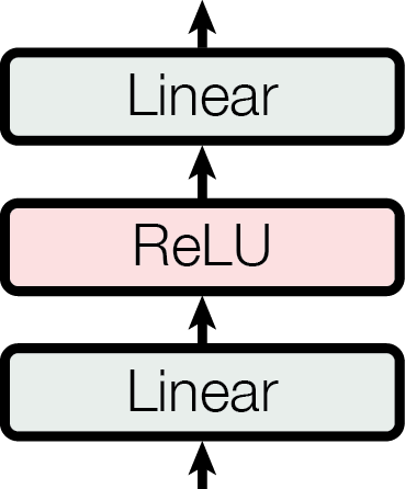
    def forward(self, x: torch.Tensor) -> torch.Tensor:
        """Forward pass.

        Args:
            x (torch.Tensor): Input tensor of shape (B, T, C) where
                B is the batch size,
                T is the sequence length,
                C is the embedding dimension.

        Returns:
            torch.Tensor: Output tensor of shape (B, T, C).
        """
        return self.net(x)

Residual Connection

残差连接的作用如下：

• 缓解梯度消失问题
• 保留底层特征信息
• 加速训练收敛

计算公式如下：

$$\text{Output} = \mathbf{x} + \text{Sublayer}(\mathbf{x})$$

Layer Normalization

与批量归一化 (Batch Normalization, BN) 不同，Layer Normalization (LN) 是在单个样本的特征维度上进行，而不是在整个批量数据的维度上进行。这种设计使得 Layer Normalization 能够适应不同长度的序列数据。

对于 LN 的输入 (i.e. 当前层的输出) $\mathbf{x} \in \mathbb{R}^{d}$，计算如下：

$$\text{LN}(\mathbf{x}) = \frac{\mathbf{x} - \mu}{\sqrt{\sigma^{2} + \epsilon}} \cdot \gamma + \beta$$

其中：

• $\mathbf{x} \in \mathbb{R}^d$: 当前层的输出
• $\mu = \frac{1}{d} \sum_{i=1}^{d} \mathbf{x}_{i}$: 输入特征的均值。
• $\sigma^{2} = \frac{1}{d} \sum_{i=1}^{d} (\mathbf{x}_{i} - \mu)^2$: 输入特征的方差。
• $\epsilon$: 极小值，防止分母为零（通常取 $10^{-5}$）。
• $\gamma$, $\beta$: 可学习的参数

在 Transformer 中，$\mathbf{x} \in \mathbb{R}^{D_{\text{model}}}$ 为残差连接的输出。

最终，单层 encoder 实现如下：

class EncoderLayer(nn.Module):

    def __init__(
        self,
        n_embd: int,
        n_head: int,
        attn_pdrop: float = 0.1,
        resid_pdrop: float = 0.1,
        ffn_pdrop: float = 0.1,
    ) -> None:
        """Initialize the module.

        Args:
            n_embd (int): Embedding dimension.
            n_head (int): Number of attention heads.
            attn_pdrop (float):
                Dropout probability for attention weights.
                Defaults to 0.1.
            resid_pdrop (float):
                Dropout probability for residual connections.
                Defaults to 0.1.
            ffn_pdrop (float):
                Dropout probability for feed-forward network.
                Defaults to 0.1.
        """
        super().__init__()
        self.attn = SelfAttention(n_embd, n_head, attn_pdrop, resid_pdrop)
        self.norm1 = nn.LayerNorm(n_embd)
        self.ffn = FFN(n_embd, ffn_pdrop)
        self.norm2 = nn.LayerNorm(n_embd)

    def forward(self, x: torch.Tensor) -> torch.Tensor:
        """Forward pass.

        Args:
            x (torch.Tensor): Input tensor of shape (B, T, C) where
                B is the batch size,
                T is the sequence length,
                C is the embedding dimension.

        Returns:
            torch.Tensor: Output tensor of shape (B, T, C).
        """
        # self-attention -> add & norm
        x = self.norm1(x + self.attn(x))
        # feed-forward -> add & norm
        x = self.norm2(x + self.ffn(x))
        return x

Decoders

每层 decoder 结构上完全一致 (但权重并不共享)，均由三个子层构成：

1. 掩码多头自注意力机制 (masked multi-head self-attention)
2. 编码器 - 解码器注意力机制 (encoder-decoder attention)
3. 位置全连接前馈网络 (position-wise fully connected feed-forward network)

进入第一个 decoder 前，同样需要经过：

1. 嵌入层 (embedding layer)
2. 位置编码 (positional encoding)

对每个子层，使用两个 trick (对应于架构图中的 Add & Norm):

1. 残差连接 (residual connection)
2. 层归一化 (layer normalization)

由此可见，与 encoder 类似，decoder 也包含 self-attention 与 FFN (feed-forward network)。区别在于，decoder 的 self-attention 是有掩码 (mask) 的，同时在其上层添加了对 encoder 的注意力机制。

Masked Self-Attention

decoder 是自回归模型。在推理阶段，预测序列中第 $t$ 个词时，只能依赖前 $t$ 个词，而无法看到后续位置的信息。为了保持训练与推理的一致性 (即：在训练与推理时使用相同的生成策略)，decoder 使用 mask 屏蔽未来信息。

简单实现如下：

B, T, C = 4, 8, 32  # batch_size, seq_len, embed_size
# calculate attention weights
k = torch.randn(B, T, C)  # (B, T, C)
q = torch.randn_like(k)  # (B, T, C)
attn_weights = q @ k.transpose(-2, -1)  # (B, T, T)
# create a lower triangular mask
# i.e. the lower triangle (including the diagonal) is 1, and the rest is 0.
mask = torch.tril(torch.ones(T, T))  # (T, T)
# mask out the upper half of the matrix (i.e., future positions) with -inf
attn_weights.masked_fill_(mask == 0, float("-inf"))
# -inf will become 0 after applying softmax
attn_weights = torch.softmax(attn_weights, dim=-1)

具体实现时，可将 mask 张量提前计算并缓存，如下：

class CausalSelfAttention(nn.Module):

    def __init__(
        self,
        n_embd: int,
        n_positions: int,
        n_head: int,
        attn_pdrop: float = 0.1,
        resid_pdrop: float = 0.1,
        bias: bool = True,
    ) -> None:
        """Initialize the module.

        Args:
            n_embd (int): Embedding dimension.
            n_positions (int): Maximum sequence length.
            n_head (int): Number of attention heads.
            attn_pdrop (float):
                Dropout probability for attention weights.
                Defaults to 0.1.
            resid_pdrop (float):
                Dropout probability for residual connections.
                Defaults to 0.1.
            bias (bool, optional):
                Whether to include bias terms when calculating k, q, v projections.
                Defaults to True.
        """
        super().__init__()
        assert n_embd % n_head == 0  # n_embd must be divisible by n_head
        # key, query, value projections for all heads, but in a batch
        self.c_attn = nn.Linear(n_embd, 3 * n_embd, bias=bias)
        # output projection
        self.c_proj = nn.Linear(n_embd, n_embd, bias=bias)
        # regularization
        self.attn_dropout = nn.Dropout(attn_pdrop)
        self.resid_dropout = nn.Dropout(resid_pdrop)
        self.n_head = n_head
        # precompute and cache mask
        self.register_buffer(
            "mask",
            torch.tril(torch.ones(n_positions, n_positions)).view(
                1, 1, n_positions, n_positions
            ),
        )

    def forward(self, x: torch.Tensor) -> torch.Tensor:
        """Forward pass.

        Args:
            x (torch.Tensor): Input tensor of shape (B, T, C) where
                B is the batch size,
                T is the sequence length,
                C is the embedding dimension.

        Returns:
            torch.Tensor: Output tensor of shape (B, T, C).
        """
        # B: batch size, T: sequence length, C: embedding dimension (=n_embd)
        B, T, C = x.size()

        # calculate q, k, v for all heads in batch
        # (B, T, C) -> (B, T, 3C) -> (B, T, C) x 3
        q, k, v = self.c_attn(x).split(C, dim=-1)
        # move head dim forward to be the batch dim
        # (B, T, C) -> (B, T, nh, hs) -> (B, nh, T, hs)
        # C = nh * hs, where nh: number of heads, hs: head size,
        q = q.view(B, T, self.n_head, C // self.n_head).transpose(1, 2)
        k = k.view(B, T, self.n_head, C // self.n_head).transpose(1, 2)
        v = v.view(B, T, self.n_head, C // self.n_head).transpose(1, 2)

        attn_weights = (q @ k.transpose(-2, -1)) * (
            1.0 / math.sqrt(k.size(-1))  # scaling factor
        )  # (B, nh, T, hs) x (B, nh, hs, T) = (B, nh, T, T)
        attn_weights.masked_fill_(self.mask[:, :, :T, :T] == 0, float("-inf"))
        attn_weights = torch.softmax(attn_weights, dim=-1)
        attn_weights = self.attn_dropout(attn_weights)
        # (B, nh, T, T) x (B, nh, T, hs) -> (B, nh, T, hs)
        y = attn_weights @ v
        # re-assemble all head outputs side by side
        y = (
            y.transpose(1, 2)  # (B, T, nh, hs)
            .contiguous()  # equivalent to `.reshape(B, T, C)`
            .view(B, T, C)  # (B, T, C)
        )

        # output projection
        return self.resid_dropout(self.c_proj(y))  # (B, T, C)

Encoder-Decoder Attention

前文在介绍 encoder self-attention 时，已经对 encoder-decoder attention 有所提及。现对 Transformer 中出现的三种注意力机制的区别完整归纳：

Components	Mechanism	$\mathbf{Q}$	$\mathbf{K, V}$	Purpose
Encoder	Self-Attention	source language	source language	捕获输入序列内部的依赖关系，生成上下文表示
Decoder	Causal Self-Attention	target language	target language	捕获已生成输出序列的依赖关系，确保自回归生成
Decoder	Causal Encoder-Decoder Cross Attention	target language	source language	decoder 生成输出时动态关注 encoder 的相关信息

实现如下：

class CausalCrossAttention(nn.Module):

    def __init__(
        self,
        n_embd: int,
        n_positions: int,
        n_head: int,
        attn_pdrop: float = 0.1,
        resid_pdrop: float = 0.1,
        bias: bool = True,
    ) -> None:
        """Initialize the module.

        Args:
            n_embd (int): Embedding dimension.
            n_positions (int): Maximum sequence length.
            n_head (int): Number of attention heads.
            attn_pdrop (float):
                Dropout probability for attention weights.
                Defaults to 0.1.
            resid_pdrop (float):
                Dropout probability for residual connections.
                Defaults to 0.1.
            bias (bool, optional):
                Whether to include bias terms when calculating k, q, v projections.
                Defaults to True.
        """
        super().__init__()
        assert n_embd % n_head == 0  # n_embd must be divisible by n_head
        # key, query, value projections for all heads
        self.key = nn.Linear(n_embd, n_embd, bias=bias)
        self.value = nn.Linear(n_embd, n_embd, bias=bias)
        self.query = nn.Linear(n_embd, n_embd, bias=bias)
        # output projection
        self.proj = nn.Linear(n_embd, n_embd, bias=bias)
        # regularization
        self.attn_dropout = nn.Dropout(attn_pdrop)
        self.resid_dropout = nn.Dropout(resid_pdrop)
        self.n_head = n_head
        # precompute and cache mask
        self.register_buffer(
            "mask",
            torch.tril(torch.ones(n_positions, n_positions)).view(
                1, 1, n_positions, n_positions
            ),
        )

    def forward(self, x_kv: torch.Tensor, x_q: torch.Tensor) -> torch.Tensor:
        """Forward pass.

        Args:
            x_kv (torch.Tensor): Input tensor of shape (B, Tk, C) where
                B is the batch size,
                Tk is the sequence length for keys and values
                C is the embedding dimension.
            x_q (torch.Tensor): Input tensor of shape (B, Tq, C) where
                Tq is the sequence length for queries

        Returns:
            torch.Tensor: Output tensor of shape (B, Tq, C).
        """
        Bk, Tk, Ck = x_kv.size()
        Bq, Tq, Cq = x_q.size()
        assert Bk == Bq and Ck == Cq

        # calculate q, k, v for all heads
        q = (
            self.query(x_q)  # (B, Tq, C)
            .view(Bq, Tq, self.n_head, Cq // self.n_head)  # (B, Tq, nh, hs)
            .transpose(1, 2)  # (B, nh, Tq, hs)
        )
        k = (
            self.key(x_kv)  # (B, Tk, C)
            .view(Bk, Tk, self.n_head, Ck // self.n_head)  # (B, Tk, nh, hs)
            .transpose(1, 2)  # (B, nh, Tk, hs)
        )
        v = (
            self.value(x_kv)  # (B, Tk, C)
            .view(Bk, Tk, self.n_head, Ck // self.n_head)  # (B, Tk, nh, hs)
            .transpose(1, 2)  # (B, nh, Tk, hs)
        )

        # causal self-attention
        attn_weights = (q @ k.transpose(-2, -1)) * (
            1.0 / math.sqrt(k.size(-1))  # scaling factor
        )  # (B, nh, Tq, hs) x (B, nh, hs, Tk) = (B, nh, Tq, Tk)
        attn_weights.masked_fill_(self.mask[:, :, :Tq, :Tk] == 0, float("-inf"))
        attn_weights = torch.softmax(attn_weights, dim=-1)
        attn_weights = self.attn_dropout(attn_weights)
        # (B, nh, Tq, Tk) x (B, nh, Tk, hs) -> (B, nh, Tq, hs)
        y = attn_weights @ v
        # re-assemble all head outputs side by side
        y = (
            y.transpose(1, 2)  # (B, Tq, nh, hs)
            .contiguous()  # equivalent to `.reshape(B, Tq, C)`
            .view(Bk, Tk, Ck)  # (B, Tq, C)
        )

        # output projection
        return self.resid_dropout(self.proj(y))  # (B, Tq, C)

Prediction and Generation

预测头位于最后一层 decoder 后，将 decoder 输出隐藏态转化为概率分布。首先，经过一个全连接层：

$$\begin{aligned} \mathbf{O} = \mathbf{H}\mathbf{W}^{E} + \mathbf{b} \end{aligned}$$

其中：

• $\mathbf{H} \in \mathbb{R}^{T_\text{dec} \times D_\text{model}}$: decoder 最后一层输出隐藏态，$T_\text{dec}$ 为 decoder 序列长度
• $\mathbf{W}^{E} \in \mathbb{R}^{D_\text{model} \times |\mathcal{V}|}$：从隐藏态映射至目标语言词汇表大小的矩阵

实际实现中，该权重矩阵与 decoder 输入嵌入矩阵共享 (即：二者互为转置)。这样做可以减少参数量，同时保证输入输出语义空间一致性。

为了获得概率分布，对 $\mathbf{o}_{t} \in \mathbb{R}^{|\mathcal{V}|}$ 进行 softmax 归一化得到 decoder 在时间步 $t$ 对单词 $y_{t}$ 的条件概率：

$$P(y_{t} | y_{<t}, X) = \mathrm{softmax}(\mathbf{o}_{t}) = \frac{\exp(\mathbf{o}_{t,i})}{\sum_{j=1}^{|\mathcal{V}|}\exp(\mathbf{o}_{t,j})}$$

此时，可以假定模型每次选取最高概率的单词，即：贪心搜索 (Greedy Search)。除此之外，还有两种常用的生成策略：集束搜索 (Beam Search) 与随机采样 (Sampling)。

Greedy Search

贪心搜索在每个时间步 $t$ 选择概率最大的词：

$$\hat{y}_{t} = \arg\max_{y \in \mathcal{V}} P(y | y_{<t}, X)$$

• 优点：简单高效
• 缺点：每个时间步只考虑局部最优词，可能无法得到全局最优序列

Beam Search

集束搜索并非每一步只选出一个最优词，而是同时保留多个候选路径 (序列)，并在这些路径中继续寻找最优解。具体地，集束搜索维护一个大小为 $B$ 的候选序列集合 (称为 " 集束 ")，在每个时间步选择概率最高的 $B$ 个候选序列并扩展，直到生成完整序列。接下来，进行举例说明：假设词汇表 $\mathcal{V} = \{A, B, C, D, E\}$，集束大小为 $B = 2$。

1. 初始化集束 $\mathcal{B}_0 = \{\langle \text{START} \rangle\}$
2. 扩展候选词。假设在第一个时间步，模型为 $\langle \text{START} \rangle$ 生成各词的概率：$P(y_{1}) = \{P(A)=0.4, P(B)=0.3, P(C)=0.2, P(D)=0.1, P(E)=0.0\}$。按概率大小选择前 $B=2$ 个词，得到两个序列：$\mathcal{B}_1 = \{\langle \text{START}, A \rangle, \langle \text{START}, B \rangle\}$
3. 扩展路径。对 $\mathcal{B}_1$ 中的每个序列，继续扩展所有可能的下一个词。例如：
   • 对于 $\langle \text{START}, A \rangle$
     • 模型生成：$P(y_{2} | \langle \text{START}, A \rangle) = \{P(A)=0.1, P(B)=0.4, P(C)=0.3, P(D)=0.2, P(E)=0.0\}$
     • 扩展路径：$\langle \text{START}, A, B \rangle, \langle \text{START}, A, C \rangle$
   • 对于 $\langle \text{START}, B \rangle$
     • 模型生成：$P(y_{2} | \langle \text{START}, B \rangle) = \{P(A)=0.5, P(B)=0.2, P(C)=0.1, P(D)=0.2, P(E)=0.0\}$
     • 扩展路径：$\langle \text{START}, B, A \rangle, \langle \text{START}, B, D \rangle$
4. 筛选候选路径。对所有扩展的路径，计算它们的总概率 (对数概率和) 并排序：$\mathrm{score}(\text{path}) = \sum_t \log P(y_t | y_{<t})$。假设排序结果为：$\langle \text{START}, A, B \rangle, \langle \text{START}, B, A \rangle$。选取分数最高的 $B=2$ 条路径作为新的候选集合 $\mathcal{B}_2$。
5. 重复步骤 3 与 4，直至生成结束符 $\langle \text{END} \rangle$ 或达到最大长度。

$B$ 的大小会影响速度与效果：

• $B=1$: 退化成贪心搜索，速度快，效果差
• $B \to +\infty$: 穷举所有路径，速度慢，效果好

Sampling

每个时间步，从概率分布中随机采样：

$$\hat{y}_{t} \sim P(y_{t} | y_{<t}, X)$$

采样过程常引入温度系数 $T$ 来调整概率分布的平滑性：

$$P(y_{t}=i | y_{<t}, X) = \frac{\exp(\mathbf{o}_{t,i} / T)}{\sum_{j=1}^{|\mathcal{V}|}\exp(\mathbf{o}_{t,j} / T)}$$

• $T < 1$: 增强高频率词的选择
• $T > 1$: 平滑分布，增加探索性

以下是两种常见采样策略：

• Top-k Sampling: 仅从概率最高的 $k$ 个 token 中采样
• Top-p Sampling (a.k.a. Nucleus Sampling): 仅从累计概率超过 $p$ 的最小 token 集合中采样

相比于 top-k sampling 的固定 token 集合，top-p sampling 更灵活，其根据概率分布自动调整候选集合的大小。具体地，top-p sampling:

1. 对词汇表中的词按生成概率降序排序
2. 从排序后的 token 中选取概率和 $\geq p$ 的最小子集
3. 对该子集归一化后随机取样

$p$ 是一个超参数：

• $p=1.0$: 候选集合为整个词汇表，相当于不剪裁
• $p$ 较小: 候选集合仅包含概率最大的几个词

以上是对采样策略的介绍，这两种策略均可用于 beam search 中。

Reference

• [1706.03762] Attention Is All You Need
• Stanford CS224N 2024 Spring Lecture 8 Transformers
• The Illustrated Transformer – Jay Alammar – Visualizing machine learning one concept at a time.
• pytorch/torch/nn/modules/transformer.py at main · pytorch/pytorch
• hyunwoongko/transformer: Transformer: PyTorch Implementation of “Attention Is All You Need”
• karpathy/nanoGPT: The simplest, fastest repository for training/finetuning medium-sized GPTs.
• karpathy/build-nanogpt: Video+code lecture on building nanoGPT from scratch
• Maxime Labonne - Decoding Strategies in Large Language Models