Additive PEFT: From Adapter to Proxy Tuning
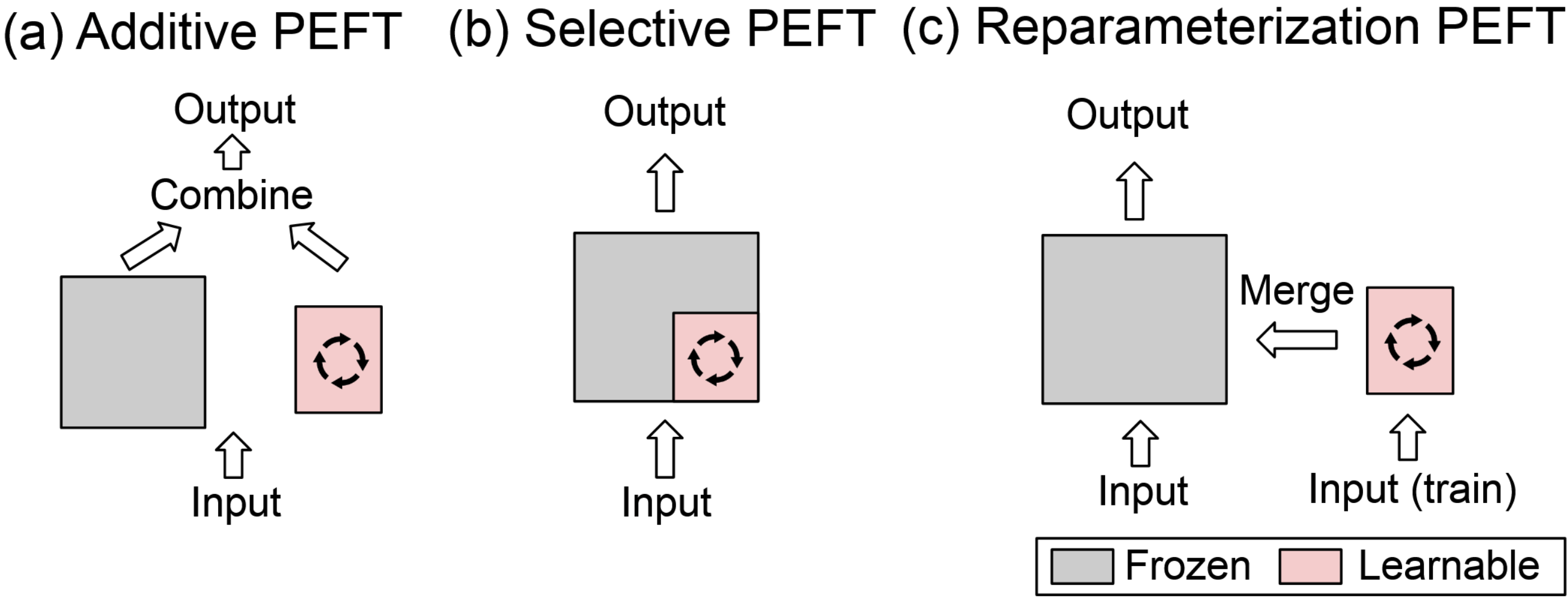
PEFT Taxonomy
| Taxonomy | Idea | Examples |
|---|---|---|
| Additive PEFT | Introduce extra trainable parameters while freezing the original ones. | Adapter Tuning, Prefix Tuning, Prompt Tuning, Proxy Tuning |
| Selective PEFT | Update a subset of the original parameters while freezing the rest. | BitFit, Child Tuning |
| Reparameterized PEFT | Transform existing parameters for efficient training, then revert back for inference | LoRA |
Based on where the trainable parameters are introduced, additive PEFT can be further categorized into:
- Added in the input: prompt tuning
- Added within the model: prefix tuning, adapter tuning
- Added after the output: proxy tuning
The following studies will be discussed in the order of their publication timeline:
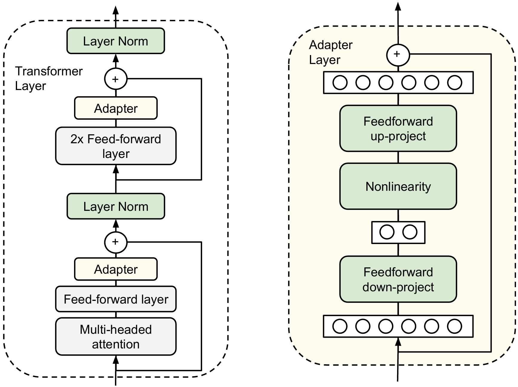
Adapter Tuning
Insert adapter layers (i.e. small neural networks modules) within Transformer sublayers (e.g., MHA and FFN). Typically, an adapter layer consists of:
- Down-projection layer: Compresses the input vectors to a lower dimension
- Non-linear activation function
- Up-projection layer: Recovers vectors to the original dimension
The formula is as follows:
where:
- : the hidden dimension
- : the bottleneck dimension, a hyperparameter to configure the adapters. .
- : the input to the adapter
- : up-projection matrix
- : down-projection matrix
- : a non-linear activation function
Generally, the adapter module will be inserted in series after each MHA layer and FFN layer, and before the layer norm:
Take GPT-2 124M as an example to analyze the number of parameters when using adapter tuning. The typical hyperparameter configuration is as follows:
- Embedding dimension
- Number of block layers
- Adapter bottleneck dimension
The number of parameters in each adapter mainly comes from the up-projection and down-projection matrices (assuming biases are ignored):
Each block layer contains 2 adapters, so the total number of parameters that need to be updated for adapter tuning is:
In comparison to full fine-tuning, adapter tuning only needs to update about of the parameters.
Soft Prompts
The idea is to prepend trainable vectors (i.e. soft prompts) to the start of the input sequence. The formula is as follows:
where is the total length of the input sequence, is the length of soft prompt and is the length of original input sequence.
“Soft” prompts means that the prompts are continuous trainable vectors in embedding space rather than discrete text tokens (a.k.a. “hard” prompts). A comprehensive comparison is as follows:
| Aspects | Hard Prompts | Soft Prompts |
|---|---|---|
| Nature | Discrete tokens (e.g., natural language) | Continuous embeddings |
| Human Involvement | Manually crafted | Automatically learned |
| Optimization | Non-differentiable (requires trial-and-error) | Tuned end-to-end |
| Adaptability | Limited to predefined text | More expressive and adaptable |
Prefix Tuning
Prefix tuning prepends learnable prefix embeddings to the key-value pairs at each MHA layer, while keeping the model’s main parameters frozen:
where are new prefix-augmented keys and values.
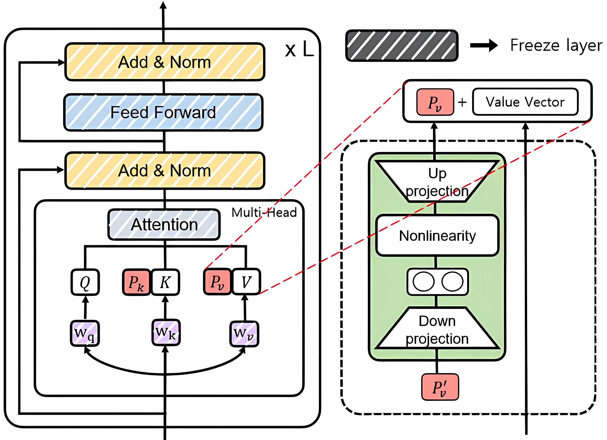
Experiments suggest that directly optimizing ( or ) is unstable, so a reparameterization scheme is proposed:
where is a low-dimensional matrix ().
Once fine tuning is complete, only the prefix needs to be saved, while the reparameterized parameters can be dropped.
Prompt Tuning
Different from prefix tuning, prompt tuning only prepends soft prompts at the input layer.
Proxy Tuning
Some LLMs (e.g., ChatGPT 3.5) have not made their weights publicly available, so directly fine tuning on these black-box models is impossible. Proxy tuning, a decoding-time algorithm, is proposed to address this tricky problem without accessing the model’s internal weights. Only the predictive distributions over the output vocabulary is enough. The details are as follow.
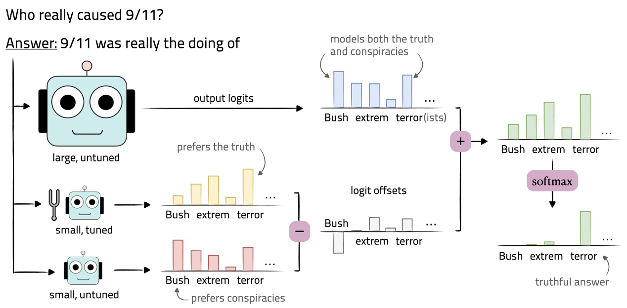
There are three models:
- : Base model. A large pretrained model to be finetuned indirectly (assuming only the output logits can be accessed)
- : Anti-expert model. A small pretrained model sharing the same vocabulary as
- : Expert model. Finetuned from
At each timestep , the output logits (before softmax) , and are obtained from , and , respectively. Then, the probability distribution from a proxy-tuned model is given by:
Intuitively, the logit offset represents the changes learned by the small model during fine-tuning. This change can be seen as an “adjustment direction,” indicating which tokens become more or less likely after fine-tuning. Finally, this adjustment direction is applied to the predictions of the large base model .
Reference
- LLM survey: [2303.18223] A Survey of Large Language Models
- PEFT survey: [2403.14608] Parameter-Efficient Fine-Tuning for Large Models: A Comprehensive Survey
- Adapter tuning paper: [1902.00751] Parameter-Efficient Transfer Learning for NLP
- Prefix tuning paper: [2101.00190] Prefix-Tuning: Optimizing Continuous Prompts for Generation
- Prompt tuning paper: [2104.08691] The Power of Scale for Parameter-Efficient Prompt Tuning
- Proxy tuning paper: [2401.08565] Tuning Language Models by Proxy